Simulation in NumPy
Simulator has NumPy implementations of the included models. Once the model is trained, experiments can be done entirely in NumPy without any reliance on TensorFlow, giving full control to researchers.
There may be some floating point error differences between NumPy and TensorFlow implementations – these grow the more timepoints the model is run on, but shouldn’t cause major issues.
Here we will demonstrate training a simple model in tensorflow, and then loading it and simulating it in NumPy.
The Simulator can be loaded either directly from a model, from saved weights in a file, or from a dictionary of weights. All options will be shown below.
[2]:
from psychrnn.backend.models.basic import Basic
from psychrnn.backend.simulation import BasicSimulator
from psychrnn.tasks.perceptual_discrimination import PerceptualDiscrimination

import numpy as np

from matplotlib import pyplot as plt
%matplotlib inline
Load from Model
To load from a model we first need to have a model. Here we instantiate a basic model from the weights saved out by Simple Example.
[3]:
network_params = {'N_batch': 50,
                  'N_in': 2,
                  'N_out': 2,
                  'dt': 10,
                  'tau': 100,
                  'T': 2000,
                  'N_steps': 200,
                  'N_rec': 50,
                  'name': 'Basic',
                  'load_weights_path': './weights/saved_weights.npz'
                 }
tf_model = Basic(network_params)
Instantiate the simulator from the model. Because the model was originally trained as a Basic model, we will use BasicSimulator to simulate the model.
[4]:
simulator = BasicSimulator(rnn_model = tf_model)
Instantiate task to run the simulator on:
[5]:
pd = PerceptualDiscrimination(dt = 10, tau = 100, T = 2000, N_batch = 128)
Simulate Model
Simulate tf_model.test() using the simulator’s NumPy impelmentation, simulator.run_trials(x).
[6]:
x, y, mask, _ = pd.get_trial_batch()
outputs, states = simulator.run_trials(x)
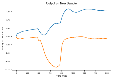
We can plot the results form the simulated model much as we could plot the results from the model in Simple Example.
[7]:
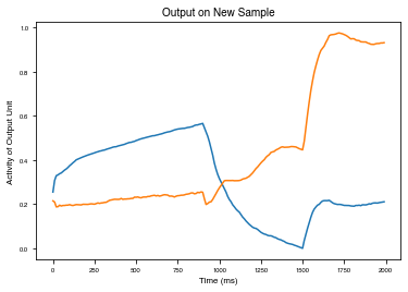
plt.plot(range(0, len(outputs[0,:,:])*10,10),outputs[0,:,:])
plt.ylabel("Activity of Output Unit")
plt.xlabel("Time (ms)")
plt.title("Output on New Sample")
[7]:
Text(0.5, 1.0, 'Output on New Sample')
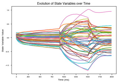
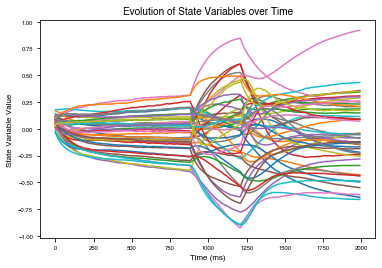
[8]:
plt.plot(range(0, len(states[0,:,:])*10,10),states[0,:,:])
plt.ylabel("State Variable Value")
plt.xlabel("Time (ms)")
plt.title("Evolution of State Variables over Time")
[8]:
Text(0.5, 1.0, 'Evolution of State Variables over Time')
[9]:
tf_model.destruct()
Load from File
Instantiate the simulator from the weights saved to file. Because the model was originally trained as a Basic model, we will use BasicSimulator to simulate the model.
[10]:
simulator = BasicSimulator(weights_path='./weights/saved_weights.npz', params = {'dt': 10, 'tau': 100})
Instantiate task to run the simulator on:
[11]:
pd = PerceptualDiscrimination(dt = 10, tau = 100, T = 2000, N_batch = 128)
Simulate Model
Simulate tf_model.test() using the simulator’s NumPy impelmentation, simulator.run_trials(x).
[12]:
x, y, mask, _ = pd.get_trial_batch()
outputs, states = simulator.run_trials(x)
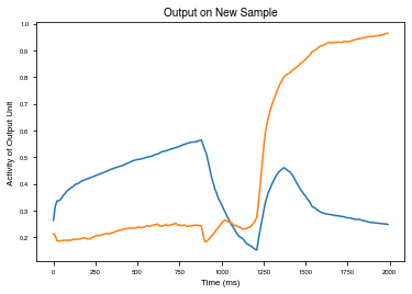
We can plot the results form the simulated model much as we could plot the results from the model in Simple Example.
[13]:
plt.plot(range(0, len(outputs[0,:,:])*10,10),outputs[0,:,:])
plt.ylabel("Activity of Output Unit")
plt.xlabel("Time (ms)")
plt.title("Output on New Sample")
[13]:
Text(0.5, 1.0, 'Output on New Sample')
[14]:
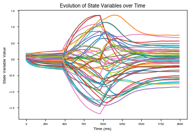
plt.plot(range(0, len(states[0,:,:])*10,10),states[0,:,:])
plt.ylabel("State Variable Value")
plt.xlabel("Time (ms)")
plt.title("Evolution of State Variables over Time")
[14]:
Text(0.5, 1.0, 'Evolution of State Variables over Time')
Load from Dictionary
Instantiate the simulator from a dictionary of weights. Because the model was originally trained as a Basic model, we will use BasicSimulator to simulate the model.
[15]:
weights = dict(np.load('./weights/saved_weights.npz', allow_pickle = True))
simulator = BasicSimulator(weights = weights , params = {'dt': 10, 'tau': 100})
Instantiate task to run the simulator on:
[16]:
pd = PerceptualDiscrimination(dt = 10, tau = 100, T = 2000, N_batch = 128)
Simulate Model
Simulate tf_model.test() using the simulator’s NumPy impelmentation, simulator.run_trials(x).
[17]:
x, y, mask, _ = pd.get_trial_batch()
outputs, states = simulator.run_trials(x)
We can plot the results form the simulated model much as we could plot the results from the model in Simple Example.
[18]:
plt.plot(range(0, len(outputs[0,:,:])*10,10),outputs[0,:,:])
plt.ylabel("Activity of Output Unit")
plt.xlabel("Time (ms)")
plt.title("Output on New Sample")
[18]:
Text(0.5, 1.0, 'Output on New Sample')
[19]:
plt.plot(range(0, len(states[0,:,:])*10,10),states[0,:,:])
plt.ylabel("State Variable Value")
plt.xlabel("Time (ms)")
plt.title("Evolution of State Variables over Time")
[19]:
Text(0.5, 1.0, 'Evolution of State Variables over Time')